We investigated gender disparity in question-asking using two lines of evidence: by collecting observational data on question-asking behaviour during 24/67 question & answer (Q&A) sessions and through self-reports on question asking collected in the post-congress survey.
3.1 Observational data
To identify a gender disparity in question asking behaviour from the observational data, we fitted a binomial generalized linear mixed effect model (GLMM), where the dependent variable indicates whether a question was asked by a woman (1) or a man (0), while accounting for the gender proportion of the audience and the nonindependence of talks within a session.
First, let’s have a look at the data used to build this model. To answer this research question, we only focus on a subset of the data: those sessions that were unmanipulated, and we excluded questions that were a follow up question from the same person, asked without raising a hand first, and asked by the host. Before building the model, we make sure that some variables such as the day, room number, the duration of the Q&A, whether a talk was given as part of the general sessions or symposia, talk number within a session, and question number was not associated with the gender of the quesioner.
Lastly, we repeat the analysis with a conserved dataset that excludes any data that had some type of uncertainty.
3.1.1 Preparing data and validation of potential covariates
# subset datadata_control <-subset(data_analysis, treatment =="Control"&is.na(followup) &is.na(jumper)&is.na(host_asks) &!grepl("speaker|questioner", allocator_question))data_control <-droplevels(data_control)# second dataset to test robustness to data with uncertaintydata_conserved <-subset(data_control, uncertainty_count_audience ==0& uncertainty_count_hands ==0)# explore datadata_control %>%select(c(session_id, talk_nr, question_nr, talk_id, gender_questioner_female, audience_total, audience_women_prop)) %>%str()
# how many questions were asked by women (1) and men (0) per session?table(data_control$session_id, data_control$gender_questioner_female) %>%kbl() %>%kable_classic_2()
0
1
4
9
12
6
5
6
15
10
11
22
6
11
25
8
6
26
10
6
28
9
6
32
9
4
34
11
6
36
10
8
37
11
7
42
0
2
44
5
7
45
12
12
48
9
8
55
8
5
61
13
5
63
4
12
69
4
3
74
10
9
80
5
6
81
3
7
83
10
12
86
5
3
# validation some potential confounding variablessummary(glmer(gender_questioner_female ~ symp_general + (1|session_id/talk_id), family ="binomial", offset=boot::logit(audience_women_prop), data = data_control)) #NS
Generalized linear mixed model fit by maximum likelihood (Laplace
  Approximation) [glmerMod]
 Family: binomial  ( logit )
Formula: gender_questioner_female ~ symp_general + (1 | session_id/talk_id)
   Data: data_control
 Offset: boot::logit(audience_women_prop)

     AIC      BIC   logLik deviance df.resid
   482.4    497.8   -237.2    474.4      346

Scaled residuals:
    Min      1Q  Median      3Q     Max
-1.5200 -0.9364 -0.7031  1.0215  1.5987

Random effects:
 Groups             Name        Variance Std.Dev.
 talk_id:session_id (Intercept) 1e-14    1e-07
 session_id         (Intercept) 0e+00    0e+00
Number of obs: 350, groups:  talk_id:session_id, 127; session_id, 24

Fixed effects:
                      Estimate Std. Error z value Pr(>|z|)
(Intercept)            -0.8677     0.1856  -4.675 2.94e-06 ***
symp_generalSymposium   0.3189     0.2293   1.391    0.164
---
Signif. codes:  0 '***' 0.001 '**' 0.01 '*' 0.05 '.' 0.1 ' ' 1

Correlation of Fixed Effects:
            (Intr)
symp_gnrlSy -0.809
optimizer (Nelder_Mead) convergence code: 0 (OK)
boundary (singular) fit: see help('isSingular')
summary(glmer(gender_questioner_female ~ talk_nr + (1|session_id/talk_id), family ="binomial", offset=boot::logit(audience_women_prop), data = data_control)) #NS
Generalized linear mixed model fit by maximum likelihood (Laplace
  Approximation) [glmerMod]
 Family: binomial  ( logit )
Formula: gender_questioner_female ~ talk_nr + (1 | session_id/talk_id)
   Data: data_control
 Offset: boot::logit(audience_women_prop)

     AIC      BIC   logLik deviance df.resid
   483.7    499.1   -237.8    475.7      346

Scaled residuals:
    Min      1Q  Median      3Q     Max
-1.6121 -0.9172 -0.6996  1.0542  1.5194

Random effects:
 Groups             Name        Variance Std.Dev.
 talk_id:session_id (Intercept) 0        0
 session_id         (Intercept) 0        0
Number of obs: 350, groups:  talk_id:session_id, 127; session_id, 24

Fixed effects:
            Estimate Std. Error z value Pr(>|z|)
(Intercept) -0.82656    0.23666  -3.493 0.000478 ***
talk_nr      0.04764    0.05991   0.795 0.426537
---
Signif. codes:  0 '***' 0.001 '**' 0.01 '*' 0.05 '.' 0.1 ' ' 1

Correlation of Fixed Effects:
        (Intr)
talk_nr -0.888
optimizer (Nelder_Mead) convergence code: 0 (OK)
boundary (singular) fit: see help('isSingular')
summary(glmer(gender_questioner_female ~ question_nr + (1|session_id/talk_id), family ="binomial", offset=boot::logit(audience_women_prop), data = data_control)) #NS
Generalized linear mixed model fit by maximum likelihood (Laplace
  Approximation) [glmerMod]
 Family: binomial  ( logit )
Formula: gender_questioner_female ~ question_nr + (1 | session_id/talk_id)
   Data: data_control
 Offset: boot::logit(audience_women_prop)

     AIC      BIC   logLik deviance df.resid
   484.3    499.7   -238.1    476.3      346

Scaled residuals:
    Min      1Q  Median      3Q     Max
-1.5876 -0.9170 -0.7136  1.0321  1.4711

Random effects:
 Groups             Name        Variance  Std.Dev.
 talk_id:session_id (Intercept) 4.949e-16 2.225e-08
 session_id         (Intercept) 0.000e+00 0.000e+00
Number of obs: 350, groups:  talk_id:session_id, 127; session_id, 24

Fixed effects:
            Estimate Std. Error z value Pr(>|z|)
(Intercept) -0.69176    0.20582  -3.361 0.000777 ***
question_nr  0.01258    0.06845   0.184 0.854147
---
Signif. codes:  0 '***' 0.001 '**' 0.01 '*' 0.05 '.' 0.1 ' ' 1

Correlation of Fixed Effects:
            (Intr)
question_nr -0.849
optimizer (Nelder_Mead) convergence code: 0 (OK)
boundary (singular) fit: see help('isSingular')
summary(glmer(gender_questioner_female ~ no_observers + (1|session_id/talk_id), family ="binomial", offset=boot::logit(audience_women_prop), data = data_control)) #NS
Generalized linear mixed model fit by maximum likelihood (Laplace
  Approximation) [glmerMod]
 Family: binomial  ( logit )
Formula: gender_questioner_female ~ no_observers + (1 | session_id/talk_id)
   Data: data_control
 Offset: boot::logit(audience_women_prop)

     AIC      BIC   logLik deviance df.resid
   483.4    498.8   -237.7    475.4      346

Scaled residuals:
    Min      1Q  Median      3Q     Max
-1.6128 -0.9208 -0.7088  1.0663  1.5360

Random effects:
 Groups             Name        Variance  Std.Dev.
 talk_id:session_id (Intercept) 2.089e-16 1.445e-08
 session_id         (Intercept) 0.000e+00 0.000e+00
Number of obs: 350, groups:  talk_id:session_id, 127; session_id, 24

Fixed effects:
             Estimate Std. Error z value Pr(>|z|)
(Intercept)   -0.8709     0.2447  -3.559 0.000372 ***
no_observers   0.1179     0.1222   0.965 0.334629
---
Signif. codes:  0 '***' 0.001 '**' 0.01 '*' 0.05 '.' 0.1 ' ' 1

Correlation of Fixed Effects:
            (Intr)
no_observrs -0.896
optimizer (Nelder_Mead) convergence code: 0 (OK)
boundary (singular) fit: see help('isSingular')
summary(glmer(gender_questioner_female ~ duration_qa + (1|session_id/talk_id), family ="binomial", offset=boot::logit(audience_women_prop), data = data_control)) #NS
Generalized linear mixed model fit by maximum likelihood (Laplace
  Approximation) [glmerMod]
 Family: binomial  ( logit )
Formula: gender_questioner_female ~ duration_qa + (1 | session_id/talk_id)
   Data: data_control
 Offset: boot::logit(audience_women_prop)

     AIC      BIC   logLik deviance df.resid
   441.5    456.5   -216.7    433.5      315

Scaled residuals:
    Min      1Q  Median      3Q     Max
-1.5755 -0.9050 -0.7259  0.9971  1.4105

Random effects:
 Groups             Name        Variance Std.Dev.
 talk_id:session_id (Intercept) 0        0
 session_id         (Intercept) 0        0
Number of obs: 319, groups:  talk_id:session_id, 118; session_id, 24

Fixed effects:
            Estimate Std. Error z value Pr(>|z|)
(Intercept) -1.01371    0.28644  -3.539 0.000402 ***
duration_qa  0.08294    0.05720   1.450 0.147087
---
Signif. codes:  0 '***' 0.001 '**' 0.01 '*' 0.05 '.' 0.1 ' ' 1

Correlation of Fixed Effects:
            (Intr)
duration_qa -0.917
optimizer (Nelder_Mead) convergence code: 0 (OK)
boundary (singular) fit: see help('isSingular')
summary(glmer(gender_questioner_female ~ time + (1|session_id/talk_id), family ="binomial", offset=boot::logit(audience_women_prop), data = data_control)) #NS
Generalized linear mixed model fit by maximum likelihood (Laplace
  Approximation) [glmerMod]
 Family: binomial  ( logit )
Formula: gender_questioner_female ~ time + (1 | session_id/talk_id)
   Data: data_control
 Offset: boot::logit(audience_women_prop)

     AIC      BIC   logLik deviance df.resid
   483.6    499.0   -237.8    475.6      346

Scaled residuals:
    Min      1Q  Median      3Q     Max
-1.4985 -0.9274 -0.7079  0.9989  1.5317

Random effects:
 Groups             Name        Variance Std.Dev.
 talk_id:session_id (Intercept) 1e-14    1e-07
 session_id         (Intercept) 0e+00    0e+00
Number of obs: 350, groups:  talk_id:session_id, 127; session_id, 24

Fixed effects:
            Estimate Std. Error z value Pr(>|z|)
(Intercept)  -0.7822     0.1779  -4.397  1.1e-05 ***
timeMorning   0.1966     0.2250   0.874    0.382
---
Signif. codes:  0 '***' 0.001 '**' 0.01 '*' 0.05 '.' 0.1 ' ' 1

Correlation of Fixed Effects:
            (Intr)
timeMorning -0.791
optimizer (Nelder_Mead) convergence code: 0 (OK)
boundary (singular) fit: see help('isSingular')
3.1.2 Build model
Nothing is significant, so let’s build the model
m_qa_general <-glmer(gender_questioner_female ~1+ (1|session_id/talk_id), family ="binomial", offset=boot::logit(audience_women_prop), data = data_control)# model outputsummary(m_qa_general)
Generalized linear mixed model fit by maximum likelihood (Laplace
  Approximation) [glmerMod]
 Family: binomial  ( logit )
Formula: gender_questioner_female ~ 1 + (1 | session_id/talk_id)
   Data: data_control
 Offset: boot::logit(audience_women_prop)

     AIC      BIC   logLik deviance df.resid
   482.3    493.9   -238.2    476.3      347

Scaled residuals:
    Min      1Q  Median      3Q     Max
-1.5932 -0.9173 -0.7136  1.0366  1.4660

Random effects:
 Groups             Name        Variance  Std.Dev.
 talk_id:session_id (Intercept) 2.603e-15 5.102e-08
 session_id         (Intercept) 0.000e+00 0.000e+00
Number of obs: 350, groups:  talk_id:session_id, 127; session_id, 24

Fixed effects:
            Estimate Std. Error z value Pr(>|z|)
(Intercept)  -0.6597     0.1088  -6.065 1.32e-09 ***
---
Signif. codes:  0 '***' 0.001 '**' 0.01 '*' 0.05 '.' 0.1 ' ' 1
optimizer (Nelder_Mead) convergence code: 0 (OK)
boundary (singular) fit: see help('isSingular')
# use helper function to collect model output in data framem_qa_general_out <-collect_out(model = m_qa_general, null =NA, name ="QA_justIC", n_factors =0, type ="qa", save="yes", dir="../results/question-asking/")m_qa_general_out %>%t() %>%kbl() %>%kable_classic_2()
model_name
QA_justIC
AIC
482.331
n_obs
350
lrt_pval
NA
lrt_chisq
NA
intercept_estimate
-0.66
intercept_estimate_prop
0.341
intercept_pval
0
intercept_ci_lower
-0.873
intercept_ci_higher
-0.447
n_factors
0
Looking at the model output, The probability that a woman asks a question is 34.082 % while taking into account the gender proportion of the audience. The null hypothesis therefore predicts that this probability is around 50%
3.2 Plenary sessions
We repeated the analysis above with data collected during plenary sessions (N = 11) only. During plenary sessions, we only collected data on the gender of people asking questions, as we could not count the audience reliability due to the size of the room. Instead, we use the proportion of women who registered for the congress to correct for the gender proportions in the audience.
# model similar to abovem_plenary <-glmer(questioner_female ~1+ (1|session_id), data = plenary,offset = boot::logit(prop_audience_female), family ="binomial")summary(m_plenary)
Generalized linear mixed model fit by maximum likelihood (Laplace
  Approximation) [glmerMod]
 Family: binomial  ( logit )
Formula: questioner_female ~ 1 + (1 | session_id)
   Data: plenary
 Offset: boot::logit(prop_audience_female)

     AIC      BIC   logLik deviance df.resid
    75.5     79.7    -35.8     71.5       58

Scaled residuals:
    Min      1Q  Median      3Q     Max
-0.6458 -0.6340 -0.6099  1.5484  1.6361

Random effects:
 Groups     Name        Variance Std.Dev.
 session_id (Intercept) 0.04703  0.2169
Number of obs: 60, groups:  session_id, 10

Fixed effects:
            Estimate Std. Error z value Pr(>|z|)
(Intercept)  -1.5360     0.3106  -4.945 7.61e-07 ***
---
Signif. codes:  0 '***' 0.001 '**' 0.01 '*' 0.05 '.' 0.1 ' ' 1
# helper function to collect output m_plenary_out <-collect_out(model = m_plenary, null =NA, name ="QA_plenary_justIC", n_factors =0,type ="qa", save="yes", dir="../results/question-asking/")m_plenary_out %>%t() %>%kbl() %>%kable_classic_2()
model_name
QA_plenary_justIC
AIC
75.515
n_obs
60
lrt_pval
NA
lrt_chisq
NA
intercept_estimate
-1.536
intercept_estimate_prop
0.177
intercept_pval
0
intercept_ci_lower
-2.418
intercept_ci_higher
-0.927
n_factors
0
# we don't have enough power to present the output of the following model, but as a curiosity we wondered if the gender disparity changed depending on the gender of the speakersummary(glmer(questioner_female ~ speaker_pronoun + (1|session_id), data = plenary,offset = boot::logit(prop_audience_female), family ="binomial"))
Generalized linear mixed model fit by maximum likelihood (Laplace
  Approximation) [glmerMod]
 Family: binomial  ( logit )
Formula: questioner_female ~ speaker_pronoun + (1 | session_id)
   Data: plenary
 Offset: boot::logit(prop_audience_female)

     AIC      BIC   logLik deviance df.resid
    75.0     81.3    -34.5     69.0       57

Scaled residuals:
    Min      1Q  Median      3Q     Max
-0.8528 -0.5303 -0.5303  1.1726  1.8856

Random effects:
 Groups     Name        Variance Std.Dev.
 session_id (Intercept) 0        0
Number of obs: 60, groups:  session_id, 10

Fixed effects:
                       Estimate Std. Error z value Pr(>|z|)
(Intercept)             -0.9165     0.4647  -1.972   0.0486 *
speaker_pronounShe/her  -0.9501     0.5986  -1.587   0.1125
---
Signif. codes:  0 '***' 0.001 '**' 0.01 '*' 0.05 '.' 0.1 ' ' 1

Correlation of Fixed Effects:
            (Intr)
spkr_prnnS/ -0.776
optimizer (Nelder_Mead) convergence code: 0 (OK)
boundary (singular) fit: see help('isSingular')
# although not significant, the gender bias seems to get worse when the speaker is female (intercept more negative)
3.3 Self-reports
Similarly, we identified a gender disparity in question asking using the self-reports from the post-congress survey by fitting a binomial generalized linear model (GLM), using the binomial response to the question “Did you ask a question at the congress” (1 = yes, 0 = no) as the dependent variable and the self-reported gender identity (woman, man, non-binary, other) as the independent variable.
First, let’s look at the data structure. Due to the difference in data structure, here we include gender as a fixed effect and assess the performance of this model compared to the null model (just the intercept) with a likelihood-ratio test.
  id gender pronoun         age ask_questions
1  1   Male  He/him  < 35 years            No
2  2   Male  He/him  > 50 years           Yes
3  3   Male  He/him 35-50 years           Yes
4  4   Male  He/him  < 35 years            No
5  5 Female She/her 35-50 years            No
6  6   Male  He/him  < 35 years            No
# reorder factorssurvey$gender <-factor(survey$gender, levels =c("Male", "Female", "Non-binary"))# build modelsurvey_qa_null <-glm(ask_questions ~1, data =subset(survey, !is.na(gender)), family ="binomial")survey_qa <-glm(ask_questions ~ gender, data =subset(survey, !is.na(gender)), family ="binomial")summary(survey_qa)
Call:
glm(formula = ask_questions ~ gender, family = "binomial", data = subset(survey,
    !is.na(gender)))

Coefficients:
                 Estimate Std. Error z value Pr(>|z|)
(Intercept)        0.8729     0.2073   4.212 2.54e-05 ***
genderFemale      -0.4904     0.2435  -2.014    0.044 *
genderNon-binary   0.9188     1.0998   0.835    0.403
---
Signif. codes:  0 '***' 0.001 '**' 0.01 '*' 0.05 '.' 0.1 ' ' 1

(Dispersion parameter for binomial family taken to be 1)

    Null deviance: 490.49  on 372  degrees of freedom
Residual deviance: 484.54  on 370  degrees of freedom
  (7 observations deleted due to missingness)
AIC: 490.54

Number of Fisher Scoring iterations: 4
m_survey_out <-collect_out(model = survey_qa, null = survey_qa_null, n_factors=2,name="qa_survey_general",type="survey", save ="yes", dir ="../results/question-asking/")m_survey_out %>%t() %>%kbl() %>%kable_classic_2()
model_name
qa_survey_general
AIC
490.536
n_obs
373
lrt_pval
0.051
lrt_chisq
5.958
intercept_estimate
0.873
intercept_estimate_prop
0.705
intercept_pval
0
intercept_ci_lower
0.467
intercept_ci_higher
1.279
n_factors
2
est_genderFemale
-0.49
lowerCI_genderFemale
-0.968
higherCI_genderFemale
-0.013
pval_genderFemale
0.044
zval_genderFemale
-2.014
est_genderNon-binary
0.919
lowerCI_genderNon-binary
-1.237
higherCI_genderNon-binary
3.074
pval_genderNon-binary
0.403
zval_genderNon-binary
0.835
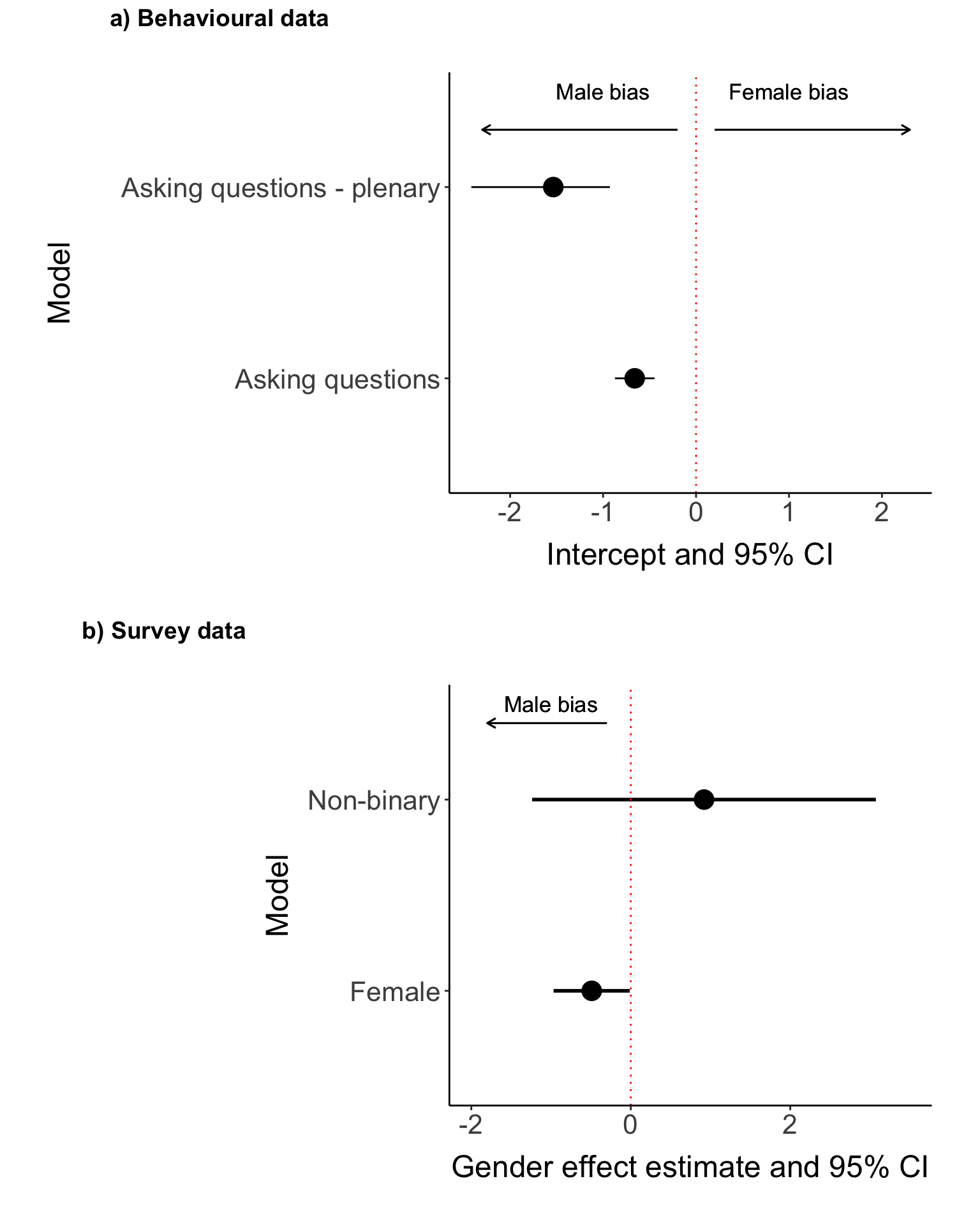
3.4 Plot output
Next, we can plot the model output in a single figure.
# combine output from all sessions and plenaries m_main_general <-rbind(m_qa_general_out, m_plenary_out)m_main_general$name <-c("Asking questions", "Asking questions - plenary") ggplot(m_main_general) +geom_point(aes(x = intercept_estimate, y = name), size =5) +geom_segment(aes(x = intercept_ci_lower, xend = intercept_ci_higher, y = name),linewidth=0.5) +geom_vline(xintercept =0, col ="red", linetype ="dotted") +labs(x ="Intercept and 95% CI", y ="Model") +geom_text(aes(label ="Male bias", y =2.5, x =-1, size =4))+geom_text(aes(label ="Female bias", y =2.5, x =1, size =4)) +geom_segment(aes(x =-0.2, xend =-2.3, y =2.3),col ="black", arrow =arrow(length=unit(0.2, "cm")))+geom_segment(aes(x =0.2, xend =2.3, y =2.3),col ="black", arrow =arrow(length=unit(0.2, "cm"))) +theme(legend.position ="none") -> plot_1_qa### also add survey# convert to include both female and non-binarym_survey_out$name <-c("Asked a question") m_survey_out_long <-data.frame(factor =c("Female", "Non-binary"),estimate =c(m_survey_out$est_genderFemale, m_survey_out$`est_genderNon-binary`),lower =c(m_survey_out$lowerCI_genderFemale, m_survey_out$`lowerCI_genderNon-binary`),upper =c(m_survey_out$higherCI_genderFemale, m_survey_out$`higherCI_genderNon-binary`))ggplot(m_survey_out_long) +geom_point(aes(x = estimate, y = factor), size =5) +geom_segment(aes(x = lower, xend = upper, y = factor),linewidth=1) +geom_vline(xintercept =0, col ="red", linetype ="dotted") +labs(x ="Gender effect estimate and 95% CI", y ="Model") +xlim(-2, 3.5) +geom_text(aes(label ="Male bias", y =2.5, x =-1, size =4))+geom_segment(aes(x =-0.3, xend =-1.8, y =2.4),col ="black", arrow =arrow(length=unit(0.2, "cm")))+theme(legend.position ="none") -> plot_2_qa_surveycowplot::plot_grid(plot_1_qa, plot_2_qa_survey, ncol =1,align ="hv", axis ="lb", labels =c("a) Behavioural data", "b) Survey data")) -> plot_qaplot_qa
3.5 Supplementary: rerun models with conservative data
As mentioned, we repeated the analysis on the observational data with the ‘conservative’ data set, which excluded any questions that some level of uncertainty in the collection. We don’t do this for the plenary sessions as the audience was not counted and any other uncertainty would have been excluded from the initial data set either way.
summary(glmer(gender_questioner_female ~1+ (1|session_id/talk_id), family ="binomial", offset=boot::logit(audience_women_prop), data = data_conserved))
Generalized linear mixed model fit by maximum likelihood (Laplace
  Approximation) [glmerMod]
 Family: binomial  ( logit )
Formula: gender_questioner_female ~ 1 + (1 | session_id/talk_id)
   Data: data_conserved
 Offset: boot::logit(audience_women_prop)

     AIC      BIC   logLik deviance df.resid
   470.6    482.2   -232.3    464.6      339

Scaled residuals:
    Min      1Q  Median      3Q     Max
-1.5818 -0.9108 -0.7139  1.0433  1.4765

Random effects:
 Groups             Name        Variance Std.Dev.
 talk_id:session_id (Intercept) 0        0
 session_id         (Intercept) 0        0
Number of obs: 342, groups:  talk_id:session_id, 124; session_id, 24

Fixed effects:
            Estimate Std. Error z value Pr(>|z|)
(Intercept)  -0.6739     0.1101  -6.122 9.25e-10 ***
---
Signif. codes:  0 '***' 0.001 '**' 0.01 '*' 0.05 '.' 0.1 ' ' 1
optimizer (Nelder_Mead) convergence code: 0 (OK)
boundary (singular) fit: see help('isSingular')
The model results seem virtually identical!
3.6 Supplementary: rerun models with only double-observed data.
Not all sessions were observed by multiple observed. To ensure the perception of gender of a single observer did not bias our conclusions, we repeated the model while excluding the sessions without a second observer.
summary(glmer(gender_questioner_female ~1+ (1|session_id/talk_id), family ="binomial", offset=boot::logit(audience_women_prop), data =subset(data_control, double_sampled =="double_sampled")))
Generalized linear mixed model fit by maximum likelihood (Laplace
  Approximation) [glmerMod]
 Family: binomial  ( logit )
Formula: gender_questioner_female ~ 1 + (1 | session_id/talk_id)
   Data: subset(data_control, double_sampled == "double_sampled")
 Offset: boot::logit(audience_women_prop)

     AIC      BIC   logLik deviance df.resid
   164.2    172.5    -79.1    158.2      116

Scaled residuals:
    Min      1Q  Median      3Q     Max
-1.4925 -0.9924  0.6700  0.9167  1.2674

Random effects:
 Groups             Name        Variance Std.Dev.
 talk_id:session_id (Intercept) 0        0
 session_id         (Intercept) 0        0
Number of obs: 119, groups:  talk_id:session_id, 46; session_id, 8

Fixed effects:
            Estimate Std. Error z value Pr(>|z|)
(Intercept)  -0.4323     0.1861  -2.323   0.0202 *
---
Signif. codes:  0 '***' 0.001 '**' 0.01 '*' 0.05 '.' 0.1 ' ' 1
optimizer (Nelder_Mead) convergence code: 0 (OK)
boundary (singular) fit: see help('isSingular')
While the results are not as extreme, likely due to reduced power by excluding sessions, they are still significant and indicate that women ask less questions than men.
3.7 Supplementary: inter-observer reliability
The data used above merge data collected by multiple observers, after we checked whether the reliability between different observers was high enough. Below you will find an example of how we calculated this IOR (inter-observer reliability) and the full script can be found under scripts/2_question_asking/ior.R.
## Example of calculating Cohen's kappa###### Host gender ####host_gender <-subset(session, !is.na(host_1_gender)) # exclude missing datawide_host_gender <-spread(host_gender[,c("session_id", "observer_talk", "host_1_gender")], observer_talk, host_1_gender)# treat observer 1 and 2 as one unit, and observer 3 and 4 as one unitwide_host_gender_a <- wide_host_gender[,c(1:3)]wide_host_gender_b <- wide_host_gender[,c(1,4,5)]names(wide_host_gender_a) <-c("session_id", "observer_a", "observer_b")names(wide_host_gender_b) <-c("session_id", "observer_a", "observer_b")# mergewide_host_gender <-rbind(wide_host_gender_a, wide_host_gender_b)# exclude sessions without double samplingwide_host_gender <-subset(wide_host_gender, !is.na(observer_a) &!is.na(observer_b)) kappa_host_gender <-kappa2(wide_host_gender[,2:3], weight ="unweighted")kappa_host_gender