5  Modelling fitness

5.1 Introduction

Now that we have mutation load (total, homozygous and heterozygous) estimates for each individual, based on SnpEff and GERP, we can model their effects on lifetime mating success (LMS).

Here, we build three sets of models:

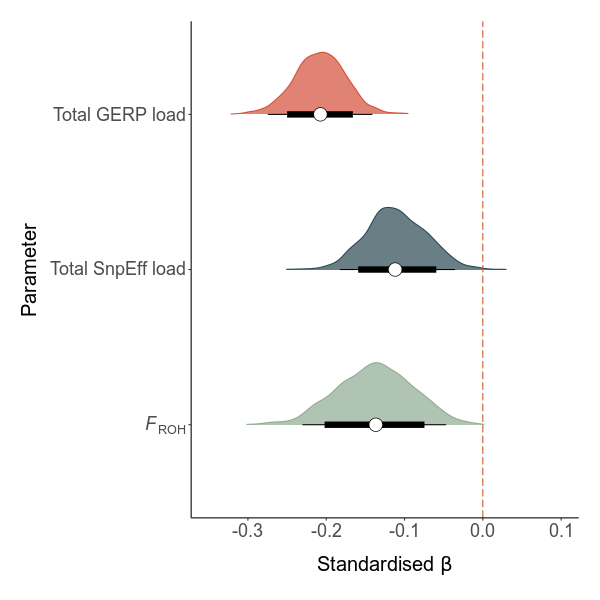
  1. The effect of total load on LMS
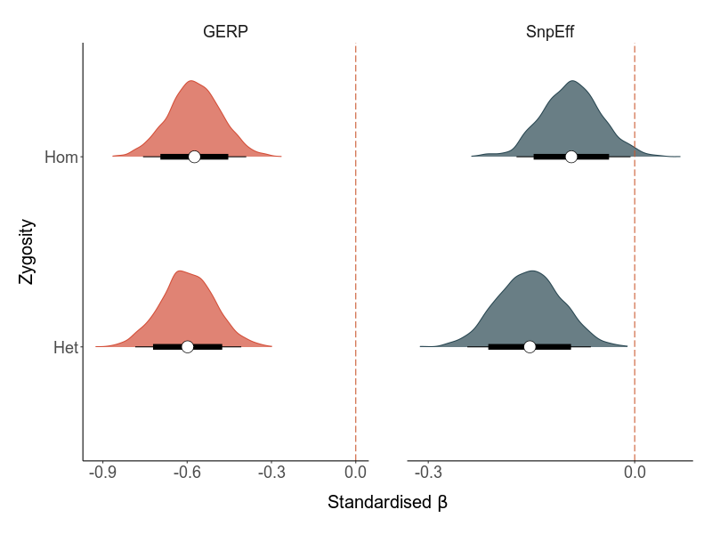
  2. The effects of homo- and heterozygous load on LMS
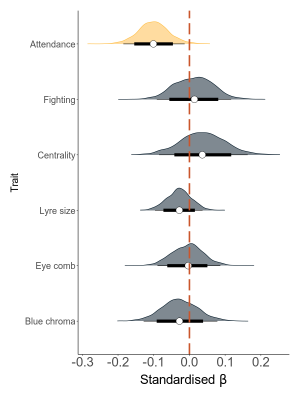
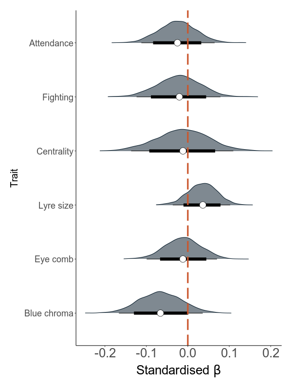
  3. The direct and indirect effects of total load on mating success through the sexual traits

We use Bayesian GLMMs using the R package ‘brms’ to compute these models

5.2 Methods

5.2.1 Total load

The general structure of the total load models is as follows:

LMS ~ scale(total_load) + core + (1|site)

To test for inbreeding depression, we ran a similar model: LMS ~ scale(froh) + core + (1|site)

This is what the script for each load type looks like:

Code
# load pheno data lifetime
load(file = "output/load/pheno_loads_lifetime.RData")

# load mutation load measures
load("output/load/all_loads_combined_da_nosex_29scaf_plus_per_region.RData") #loads no sex chr only 30 scaf

# subset only the relevant method/loadtype
load <- load_per_region %>% filter(loadtype == method)

# combine
pheno_wide_load <- left_join(pheno_wide, load, by = "id")
pheno_wide_load <- subset(pheno_wide_load, !is.na(total_load)) #some ids without genotypes, excluded for wgr

#### model ####
brm_load_t <- brm(LMS_min ~ scale(total_load) + core + (1|site), data = pheno_wide_load,
                  family = "zero_inflated_poisson",
                  prior = prior(normal(0,1), class = b),
                  cores =8, control = list(adapt_delta = 0.99, max_treedepth = 15),
                  iter = iter, thin = thin, warmup = warm, seed = 1908)

save(brm_load_t, file = out)

We can check out the performance of each model using the following loop:

Code
output_total <- list.files(path = "output/models/total_hom_het/",
                         pattern = "lms*", full.names=T)

diagnose_summary <- list()
for (i in 1:length(output)){
  #load fit
  load(file = output[[i]])
  #get posteriors
  posterior <- as.array(fit)
  log_ps <- log_posterior(fit)
  nuts <- nuts_params(fit) #divergence
  #get only beta and sd
  betas <- variables(fit)[grep("b_", variables(fit))]
  sd <- variables(fit)[grep("sd_", variables(fit))]
  
  #global patterns in divergence
  diverge_beta <- mcmc_parcoord(posterior, np = nuts, pars= betas)
  diverge_sd <- mcmc_parcoord(posterior, np = nuts, pars= sd)
  
  #identify collinearity between parameters
  collin_beta <- mcmc_pairs(posterior, np = nuts, pars= betas)
  collin_sd <- mcmc_pairs(posterior, np = nuts, pars= sd)
  
  #traceplot
  trace_beta <- mcmc_trace(posterior, pars = betas, np = nuts)
  trace_sd <- mcmc_trace(posterior, pars = sd, np = nuts)
  
  #rhat
  rhat <- mcmc_rhat(brms::rhat(fit))
  
  #effective sample size
  neff <- mcmc_neff(neff_ratio(fit))
  
  #autocorrelation
  autocor_beta <- mcmc_acf(posterior, pars = betas)
  autocor_sd <- mcmc_acf(posterior, pars=sd)
  
  #quick glance results
  areas <- mcmc_areas(fit, pars=betas)
  
  #combine in list
  diagnosis <- list(diverge_beta = diverge_beta, 
                    diverge_sd = diverge_sd, 
                    collin_beta = collin_beta, 
                    collin_sd = collin_sd, 
                    trace_beta = trace_beta, 
                    trace_sd = trace_sd, 
                    rhat = rhat, 
                    neff = neff, 
                    autocor_beta = autocor_beta, 
                    autocor_sd = autocor_sd,
                    areas = areas)
  
  
  modelname <- sub(".*/", "", output[i]) 
  modelname <- sub(".RData", "", modelname)
  
  # add to summary
  diagnose_summary[[modelname]] <- diagnosis
}

This is what these plots look like for total GERP load effects:

Diagnostics GERP total load model

5.2.2 Hom and het load

The general structure of the homozygous and heterozygous load models is as follows:

LMS ~ scale(het_load) + scale(hom_load) + core + (1|site)

This is what the script for each load type looks like:

Code
# load pheno data lifetime
load(file = "output/load/pheno_loads_lifetime.RData")

# load mutation load measures
load("output/load/all_loads_combined_da_nosex_29scaf_plus_per_region.RData") #loads no sex chr only 30 scaf

# subset only the relevant method/loadtype
load <- load_per_region %>% filter(loadtype == method)

# combine
pheno_wide_load <- left_join(pheno_wide, load, by = "id")
pheno_wide_load <- subset(pheno_wide_load, !is.na(total_load)) #some ids without genotypes, excluded for wgr

#### model ####
brm_load_het_hom <- brm(LMS_min ~ scale(het_load) + scale(hom_load) + core + (1|site), data = pheno_wide_load,
                  family = "zero_inflated_poisson",
                  prior = prior(normal(0,1), class = b),
                  cores =8, control = list(adapt_delta = 0.99, max_treedepth = 15),
                  iter = iter, thin = thin, warmup = warm, seed = 1908)

save(brm_load_het_hom, file = out)

The same diagnostics were applied to each model.

5.2.3 Direct and indirect effects

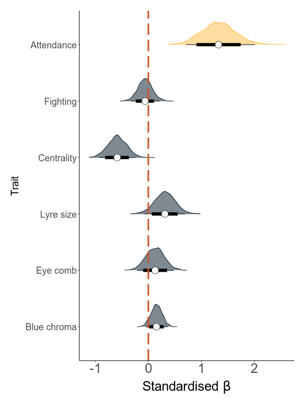
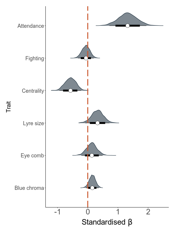
Next, we build models that are based on annual values. There are two sets of models: the first quantifies the effect of load on the six sexual traits (attendance, fighting rate, centrality, lyre size, blue chroma and red eye comb size) in six separate models. The second set analyses the effect of the six traits and load on annual mating success (MS).

The direct effect is the effect of load on MS while correcting for all mediators. The indirect effect is calculated using a mediation analysis, where this effect is calculated as the product of the effect of the predictor (the total load) on the mediator (the sexual trait) and the effect of the mediator on the response variable (AMS).

5.2.3.1 Set 1: load on traits

For each trait, we run this model:

scale(trait) ~ scale(total_load) + age_cat + (1|year) + (1|site/id)

Code
### load data ###

load(file = "data/phenotypes/phenotypes_annual.RData")

# load mutation load measures
load("output/load/all_loads_combined_da_nosex_29scaf_plus_per_region.RData") #loads no sex chr only 30 scaf

# subset only the relevant method/loadtype
load <- load_per_region %>% filter(loadtype == method)

# merge files
pheno <- left_join(pheno_long, load, by = "id")
pheno$born <- pheno$year - pheno$age
pheno <- pheno %>% mutate(age_cat = as.factor(case_when(age == 1 ~ "yearling", age > 1  ~ "adult")))

### modelling ####
formula <- formula(paste0("scale(", response, ") ~ scale(total_load) + age_cat + (1|year) + (1|site/id)"))

fit <- brm(formula,
            family = "gaussian",
           data = pheno, 
           cores =8,
           control = list(adapt_delta = 0.99, max_treedepth = 15),
           prior = prior(normal(0,1), class = b),
           iter = iterations, 
           thin = thin, warmup = burn)

save(fit, file = out)

5.2.3.2 Set 2: trait + load on MS

Then, for both approaches we run the following model:

MS ~ scale(total_load) + scale(lyre) + scale(eyec) + scale(blue) + scale(dist) + scale(attend) + scale(fight) + age_cat + (1|year) + (1|site/id)

Code
### load data ###

load(file = "data/phenotypes/phenotypes_annual.RData")

# load mutation load measures
load("output/load/all_loads_combined_da_nosex_29scaf_plus_per_region.RData") #loads no sex chr only 30 scaf

# subset only the relevant method/loadtype
load <- load_per_region %>% filter(loadtype == method)

# merge files
pheno <- left_join(pheno_long, load, by = "id")
pheno$born <- pheno$year - pheno$age

pheno <- pheno %>% mutate(age_cat = as.factor(case_when(age == 1 ~ "yearling", age > 1  ~ "adult")))

### modelling ####
formula <- formula("MS ~ scale(total_load) + scale(lyre) + scale(eyec) + scale(blue) + scale(dist) + scale(attend) + scale(fight) + age_cat + (1|year) + (1|site/id)")

fit <- brm(formula,
           family = "zero_inflated_poisson",
           data = pheno, 
           cores =8,
           control = list(adapt_delta = 0.99, max_treedepth = 15),
           prior = prior(normal(0,1), class = b),
           iter = iterations, 
           thin = thin, warmup = burn)

save(fit, file = out)

5.2.3.3 Direct / indirect effects

The direct/indirect effects are then calculated after loading in all model outputs:

Code
### load packages ####

pacman::p_load(brms, bayesplot, dplyr, data.table)

### load models ###

#### gerp ####
load(file = "output/models/annual/traits/model_attend_gerp45.RData")
fit_gerp_attend <- fit
load(file = "output/models/annual/traits/model_fight_gerp45.RData")
fit_gerp_fight <- fit
load(file = "output/models/annual/traits/model_dist_gerp45.RData")
fit_gerp_dist <- fit
load(file = "output/models/annual/traits/model_eyec_gerp45.RData")
fit_gerp_eyec <- fit
load(file = "output/models/annual/traits/model_blue_gerp45.RData")
fit_gerp_blue <- fit
load(file = "output/models/annual/traits/model_lyre_gerp45.RData")
fit_gerp_lyre <- fit

load(file = "output/models/annual/ams/model_trait_ams_gerp45.RData")
fit_gerp_ams <- fit

rm(fit)

### snpeff 
load(file = "output/models/annual/traits/model_attend_high.RData")
fit_high_attend <- fit
load(file = "output/models/annual/traits/model_fight_high.RData")
fit_high_fight <- fit
load(file = "output/models/annual/traits/model_dist_high.RData")
fit_high_dist <- fit
load(file = "output/models/annual/traits/model_eyec_high.RData")
fit_high_eyec <- fit
load(file = "output/models/annual/traits/model_blue_high.RData")
fit_high_blue <- fit
load(file = "output/models/annual/traits/model_lyre_high.RData")
fit_high_lyre <- fit

load(file = "output/models/annual/ams/model_trait_ams_high.RData")
fit_high_ams <- fit

rm(fit)

### indirect effects loop #####
get_indirect <- function(mediator, method, trait_model, ams_model){
  treatment = "b_scaletotal_load"
  path1 <- as_draws_df(trait_model, variable =treatment)
  path1 <- path1$b_scaletotal_load
  
  path2 <- as_draws_df(ams_model, variable = mediator)
  path2 <- unlist(c(path2[,1]))
  
  indirect <- path1*path2
  
  direct <- as_draws_df(ams_model, variable =treatment)
  direct <- direct$b_scaletotal_load
  
  total <- indirect + direct
  
  effect_attend <- data.frame(treatment = treatment,
                              mediator = mediator,
                              method = method,
                              indirect_median = round(median(indirect), 2),
                              indirect_lower = round(quantile(indirect, probs = c(.025)), 2),
                              indirect_upper = round(quantile(indirect, probs = c(.975)), 2),
                              direct_median = round(median(direct), 2),
                              direct_lower = round(quantile(direct, probs = c(.025)), 2),
                              direct_upper = round(quantile(direct, probs = c(.975)), 2),
                              total_median = round(median(total), 2),
                              total_lower = round(quantile(total, probs = c(.025)), 2),
                              total_upper = round(quantile(total, probs = c(.975)), 2),
                              path1_median = round(median(path1), 2),
                              path1_lower = round(quantile(path1, probs = c(.025)), 2),
                              path1_upper = round(quantile(path1, probs = c(.975)), 2),
                              path2_median = round(median(path2), 2),
                              path2_lower = round(quantile(path2, probs = c(.025)), 2),
                              path2_upper = round(quantile(path2, probs = c(.975)), 2),
                              indirect_lower_80 = round(quantile(indirect, probs = c(.1)), 2),
                              indirect_upper_80 = round(quantile(indirect, probs = c(.9)), 2),
                              direct_lower_80 = round(quantile(direct, probs = c(.1)), 2),
                              direct_upper_80 = round(quantile(direct, probs = c(.9)), 2))
  
  return(effect_attend)
}

effects <- data.frame(rbind(get_indirect(mediator="b_scalelyre", method = "gerp45", 
                                         trait_model=fit_gerp_lyre, ams_model = fit_gerp_ams),
                            get_indirect(mediator="b_scaleeyec",  method = "gerp45", 
                                         trait_model=fit_gerp_eyec, ams_model = fit_gerp_ams),
                            get_indirect(mediator="b_scaleblue",  method = "gerp45", 
                                         trait_model=fit_gerp_blue, ams_model = fit_gerp_ams),
                            get_indirect(mediator="b_scaleattend",  method = "gerp45", 
                                         trait_model=fit_gerp_attend, ams_model = fit_gerp_ams),
                            get_indirect(mediator="b_scalefight",  method = "gerp45", 
                                         trait_model=fit_gerp_fight, ams_model = fit_gerp_ams),
                            get_indirect(mediator="b_scaledist",  method = "gerp45", 
                                         trait_model=fit_gerp_dist, ams_model = fit_gerp_ams),
                            get_indirect(mediator="b_scalelyre", method = "high", 
                                         trait_model=fit_high_lyre, ams_model = fit_high_ams),
                            get_indirect(mediator="b_scaleeyec",  method = "high", 
                                         trait_model=fit_high_eyec, ams_model = fit_high_ams),
                            get_indirect(mediator="b_scaleblue",  method = "high", 
                                         trait_model=fit_high_blue, ams_model = fit_high_ams),
                            get_indirect(mediator="b_scaleattend",  method = "high", 
                                         trait_model=fit_high_attend, ams_model = fit_high_ams),
                            get_indirect(mediator="b_scalefight",  method = "high", 
                                         trait_model=fit_high_fight, ams_model = fit_high_ams),
                            get_indirect(mediator="b_scaledist",  method = "high", 
                                         trait_model=fit_high_dist, ams_model = fit_high_ams)))


write.csv(effects, file = "output/models/annual/direct_indirect_summary.csv", quote=F, row.names = F)

5.3 Results

We find significant effects of total GERP and total SnpEff load, and significant effects of inbreeding.

Total load results
Code
library(readxl); library(dplyr); library(kableExtra)
totals <- read.csv("../output/models/intervals/total_gerp45_high.csv")
totals %>% kbl() 
parameter outer_width inner_width point_est ll l m h hh model
b_scaletotal_load 0.95 0.8 median -0.27 -0.25 -0.21 -0.17 -0.14 GERP
b_scaletotal_load 0.95 0.8 median -0.18 -0.16 -0.11 -0.06 -0.04 SnpEff

We also find significant effects of both hom and het GERP and SnpEff load:

Hom het load results
Code
homhet <- read.csv("../output/models/intervals/hom_het_gerp45_high.csv")
homhet %>% kbl() 
parameter outer_width inner_width point_est ll l m h hh model loadtype
b_scalehom_load 0.95 0.8 median -0.76 -0.70 -0.57 -0.45 -0.39 Hom GERP
b_scalehet_load 0.95 0.8 median -0.78 -0.72 -0.60 -0.48 -0.41 Het GERP
b_scalehom_load 0.95 0.8 median -0.17 -0.15 -0.09 -0.04 -0.01 Hom SnpEff
b_scalehet_load 0.95 0.8 median -0.24 -0.21 -0.15 -0.09 -0.06 Het SnpEff

Here you can find the posterior distributions of model set 1 (load on traits) for GERP : MS set 1 results GERP

MS set 1 results SnpEff

And for model set 2 (traits on MS) for GERP and SnpEff: MS set 2 results GERP MS set 2 results SnpEff

We can check out the result of the direct and indirect effects as follows:

Code
effects <- read.csv("../output/models/annual/direct_indirect_summary.csv")
effects %>% kbl() %>%  kable_classic_2() %>% scroll_box(width = "99%", height = "200px")
treatment mediator method indirect_median indirect_lower indirect_upper direct_median direct_lower direct_upper total_median total_lower total_upper path1_median path1_lower path1_upper path2_median path2_lower path2_upper indirect_lower_80 indirect_upper_80 direct_lower_80 direct_upper_80
b_scaletotal_load b_scalelyre gerp45 -0.01 -0.04 0.01 -0.13 -0.36 0.11 -0.14 -0.38 0.10 -0.03 -0.10 0.04 0.31 -0.07 0.69 -0.03 0.01 -0.29 0.03
b_scaletotal_load b_scaleeyec gerp45 0.00 -0.02 0.02 -0.13 -0.36 0.11 -0.13 -0.36 0.11 0.00 -0.09 0.09 0.13 -0.21 0.48 -0.01 0.01 -0.29 0.03
b_scaletotal_load b_scaleblue gerp45 0.00 -0.03 0.01 -0.13 -0.36 0.11 -0.14 -0.38 0.10 -0.03 -0.13 0.08 0.15 -0.05 0.36 -0.02 0.01 -0.29 0.03
b_scaletotal_load b_scaleattend gerp45 -0.13 -0.28 -0.01 -0.13 -0.36 0.11 -0.26 -0.54 0.01 -0.10 -0.19 -0.01 1.32 0.71 2.01 -0.22 -0.05 -0.29 0.03
b_scaletotal_load b_scalefight gerp45 0.00 -0.02 0.02 -0.13 -0.36 0.11 -0.13 -0.36 0.11 0.01 -0.09 0.12 -0.06 -0.33 0.21 -0.01 0.01 -0.29 0.03
b_scaletotal_load b_scaledist gerp45 -0.02 -0.11 0.05 -0.13 -0.36 0.11 -0.15 -0.41 0.11 0.04 -0.09 0.16 -0.59 -0.93 -0.23 -0.07 0.02 -0.29 0.03
b_scaletotal_load b_scalelyre high 0.01 -0.01 0.05 -0.11 -0.38 0.16 -0.09 -0.37 0.18 0.04 -0.04 0.10 0.33 -0.08 0.72 0.00 0.03 -0.27 0.06
b_scaletotal_load b_scaleeyec high 0.00 -0.03 0.02 -0.11 -0.38 0.16 -0.11 -0.38 0.16 -0.01 -0.10 0.07 0.14 -0.21 0.49 -0.01 0.01 -0.27 0.06
b_scaletotal_load b_scaleblue high -0.01 -0.04 0.01 -0.11 -0.38 0.16 -0.12 -0.39 0.15 -0.07 -0.17 0.04 0.15 -0.06 0.36 -0.03 0.00 -0.27 0.06
b_scaletotal_load b_scaleattend high -0.03 -0.16 0.09 -0.11 -0.38 0.16 -0.14 -0.44 0.15 -0.03 -0.11 0.06 1.32 0.72 1.94 -0.11 0.04 -0.27 0.06
b_scaletotal_load b_scalefight high 0.00 -0.01 0.02 -0.11 -0.38 0.16 -0.10 -0.38 0.17 -0.02 -0.12 0.08 -0.06 -0.32 0.20 -0.01 0.01 -0.27 0.06
b_scaletotal_load b_scaledist high 0.01 -0.06 0.09 -0.11 -0.38 0.16 -0.10 -0.39 0.17 -0.01 -0.14 0.11 -0.57 -0.94 -0.22 -0.04 0.06 -0.27 0.06