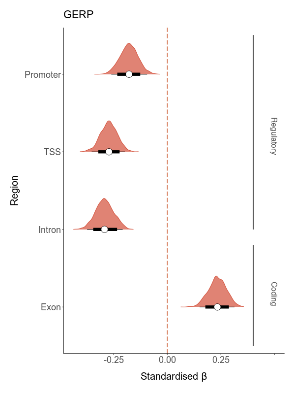
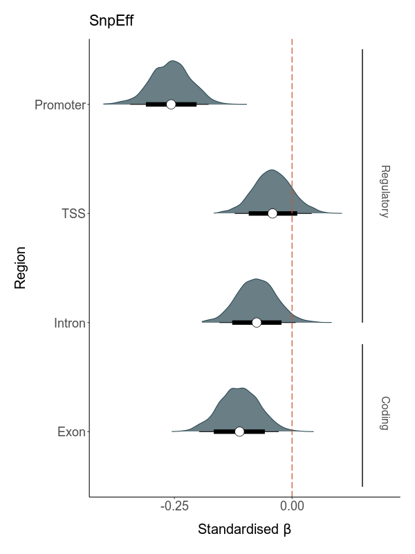
Both functional noncoding and protein-coding regions can be under selective constraint. However, the former include various regulatory elements such as promoters, enhancers and silencers, which play different roles in gene regulation and might therefore be expected to experience different strengths of purifying selection. To investigate whether the fitness effects of deleterious mutations vary by genomic region, we classified each deleterious mutation according to whether it was located within a promoter, transcription start site, intron or exon. Then, we calculate total load based on these subsets and model their effects on LMS.
6.1.1 Genomic regions
We use a combination of GenomicRanges and rtracklayer and other packages to divide up the genome annotation file into the four genomic regions.
6.1.1.1 Subset reference genome
Code
#### Packages #####pacman::p_load(BiocManager, rtracklayer, GenomicFeatures, BiocGenerics, data.table, dplyr, genomation, GenomicRanges, tibble)#### Genome data ##### first change scaffold namesgff_raw <-fread("data/genomic/annotation/PO2979_Lyrurus_tetrix_black_grouse.annotation.gff") gff_raw$V1 <-gsub(";", "__", gff_raw$V1)gff_raw$V1 <-gsub("=", "_", gff_raw$V1)write.table(gff_raw, file ="data/genomic/PO2979_Lyrurus_tetrix_black_grouse.annotation_editedscafnames.gff", sep ="\t", col.names =FALSE, quote=F, row.names =FALSE)#read in new filegff <-makeTxDbFromGFF("data/genomic/PO2979_Lyrurus_tetrix_black_grouse.annotation_editedscafnames.gff", format="gff3", organism="Lyrurus tetrix") ## divide up between the 4 regions ###promoters <-promoters(gff, upstream=2000, downstream=200, columns=c("tx_name", "gene_id")) # From NIOOTSS <-promoters(gff, upstream=300, downstream=50, columns=c("tx_name", "gene_id")) # TSS as in Laine et al., 2016. Nature Communicationsexons_gene <-unlist(exonsBy(gff, "gene")) # group exons by genesintrons <-unlist(intronsByTranscript(gff, use.names=TRUE))### write out filesexport(promoters, "data/genomic/annotation/promoters.gff3")export(TSS, "data/genomic/annotation/TSS.gff3")introns@ranges@NAMES[is.na(introns@ranges@NAMES)]<-"Unknown"export(introns, "data/genomic/annotation/introns_transcripts.gff3")export(exons_gene, "data/genomic/annotation/exons_gene.gff3")
6.1.1.2 Annotate deleterious mutations
Then, we load in all deleterious mutations for GERP and SnpEff separately and annotate the mutations according to the four regions.
Code
###### Annotate high impact and GERP mutations ######## annotate gene regions per SNP for high impact and gerp mutations ###### load data ###load(file ="output/load/snpeff/snpeff_high.RData")load(file ="output/load/gerp/gerp_over4.RData")### change scaf namessnpeff$CHROM <-gsub(";", "__", snpeff$CHROM)snpeff$CHROM <-gsub("=", "_", snpeff$CHROM)gerp$chr <-gsub(";", "__", gerp$chr)gerp$chr <-gsub("=", "_", gerp$chr)### remove genotypes: not necessary heresnpeff <- snpeff[,c(1:9)]gerp <- gerp[,c(1:9)]####### Gene regions ############## load annotation dataannotation_dir <-"data/genomic/annotation"promoter=unique(gffToGRanges(paste0(annotation_dir, "/promoters.gff3")))TSS=unique(gffToGRanges(paste0(annotation_dir, "/TSS.gff3")))introns=unique(gffToGRanges(paste0(annotation_dir, "/introns_transcripts.gff3")))exons_gene=unique(gffToGRanges(paste0(annotation_dir, "/exons_gene.gff3")))#### Annotate SNPeff regions ####snpeff$end <- snpeff$POSsnpeff$start <- snpeff$POSsnpef_gr <-as(snpeff, "GRanges")snpef_promoter <-as.data.frame(subsetByOverlaps(snpef_gr, promoter)) %>%add_column("region_promoter"=1) %>% dplyr::rename(chr = seqnames)%>%unique()snpef_TSS <-as.data.frame(subsetByOverlaps(snpef_gr, TSS))%>%add_column("region_tss"=1) %>% dplyr::rename(chr = seqnames)%>%unique()snpef_exons <-as.data.frame(subsetByOverlaps(snpef_gr, exons_gene))%>%add_column("region_exon"=1) %>% dplyr::rename(chr = seqnames)%>%unique()snpef_introns <-as.data.frame(subsetByOverlaps(snpef_gr, introns))%>%add_column("region_intron"=1) %>% dplyr::rename(chr = seqnames)%>%unique()snpef_all <-left_join(snpeff, snpef_promoter[,c("chr", "start", "region_promoter")], by =c("CHROM"="chr", "start"))%>%left_join(snpef_TSS[,c("chr", "start", "region_tss")], by =c("CHROM"="chr", "start"))%>%left_join(snpef_exons[,c("chr", "start", "region_exon")], by =c("CHROM"="chr", "start"))%>%left_join(snpef_introns[,c("chr", "start", "region_intron")], by =c("CHROM"="chr", "start"))# correct promoterssnpef_all <- snpef_all %>%mutate(region_promoter =case_when( region_tss ==1& region_promoter ==1~NA,is.na(region_tss) & region_promoter ==1~1))save(snpef_all, file ="output/load/snpeff/snpeff_high_annotated_region.RData")#### Annotate gerp regions ####gerp$end <- gerp$posgerp$start <- gerp$posgerp_gr <-as(gerp, "GRanges")gerp_promoter <-as.data.frame(subsetByOverlaps(gerp_gr, promoter)) %>%add_column("region_promoter"=1) %>% dplyr::rename(chr = seqnames)%>%unique()gerp_TSS <-as.data.frame(subsetByOverlaps(gerp_gr, TSS))%>%add_column("region_tss"=1) %>% dplyr::rename(chr = seqnames)%>%unique()gerp_exons <-as.data.frame(subsetByOverlaps(gerp_gr, exons_gene))%>%add_column("region_exon"=1) %>% dplyr::rename(chr = seqnames)%>%unique()gerp_introns <-as.data.frame(subsetByOverlaps(gerp_gr, introns))%>%add_column("region_intron"=1) %>% dplyr::rename(chr = seqnames)%>%unique()gerp_all <-left_join(gerp, gerp_promoter[,c("chr", "start", "region_promoter")], by =c("chr"="chr", "start"))%>%left_join(gerp_TSS[,c("chr", "start", "region_tss")], by =c("chr"="chr", "start"))%>%left_join(gerp_exons[,c("chr", "start", "region_exon")], by =c("chr"="chr", "start"))%>%left_join(gerp_introns[,c("chr", "start", "region_intron")], by =c("chr"="chr", "start"))# correct promotersgerp_all <- gerp_all %>%mutate(region_promoter =case_when( region_tss ==1& region_promoter ==1~NA,is.na(region_tss) & region_promoter ==1~1))save(gerp_all, file ="output/load/gerp/gerp_annotated_region.RData")
6.1.1.3 Calculate mutation load
These two files (gerp_all and snpeff_all) contain the SNP locations and additional binary columns whether the mutations was located in one of the 4 regions. We can use this file together with the files containing the genotypes to calculate mutation load based on the subsets of mutations only.
Code
#### Calculate load per region ###### load annotated gerp dataload(file ="output/load/gerp/gerp_annotated_region.RData")gerp_all$chr <-gsub("__", ";", gerp_all$chr)gerp_all$chr <-gsub("HRSCAF_", "HRSCAF=", gerp_all$chr)# load annotationload(file ="output/load/snpeff/snpeff_high_annotated_region.RData")snpef_all$CHROM <-gsub("__", ";", snpef_all$CHROM)snpef_all$CHROM <-gsub("HRSCAF_", "HRSCAF=", snpef_all$CHROM)## load functions to calculate loadsource("scripts/7_calculate_load/function_calculate_load.R")#### calculate load per region as defined below regions <-c("region_promoter", "region_tss" ,"region_exon","region_intron")#load existing combined load fileload("output/load/all_loads_combined_da_nosex_29scaf.RData") #loads no sex chr only 29 scaf# load gt again to include genotypesload(file ="output/load/snpeff/snpeff_high.RData")load(file ="output/load/gerp/gerp_over4.RData")#first gerp5load_per_region <- loadfor (region in regions){ subset_locs <-subset(gerp_all, gerp_all[,region] ==1) #subset based on region name subset_locs$chr_pos <-paste0(subset_locs$chr, "_", subset_locs$pos) #make a col for the snp position gerp$chr_pos <-paste0(gerp$chr, "_", gerp$pos) #make a col for the snp position sub_genotypes <-subset(gerp, chr_pos %in% subset_locs$chr_pos) #subset genotypes based on subset sub_genotypes$chr_pos <-NULL#remove chr_pos again loadtype =paste0("gerp45", gsub("region", "", region)) load_sub <-calculate_load_gerp(sub_genotypes, loadtype = loadtype, output_vcf = F) #calculate loads load_per_region <-rbind(load_per_region, load_sub[,c("id", "het_load", "hom_load", "total_load", "loadtype")])}#snpefffor (region in regions){ subset_locs <-subset(snpef_all, snpef_all[,region] ==1) #subset based on region name subset_locs$chr_pos <-paste0(subset_locs$CHROM, "_", subset_locs$POS) #make a col for the snp position snpeff$chr_pos <-paste0(snpeff$CHROM, "_", snpeff$POS) #make a col for the snp position sub_genotypes <-subset(snpeff, chr_pos %in% subset_locs$chr_pos) #subset genotypes based on subset sub_genotypes$chr_pos <-NULL#remove chr_pos again loadtype =paste0("high", gsub("region", "", region)) load_sub <-calculate_load_snpeff(sub_genotypes, loadtype = loadtype, output_vcf = F) #calculate loads load_per_region <-rbind(load_per_region, load_sub[,c("id", "het_load", "hom_load", "total_load", "loadtype")])}save(load_per_region, file ="output/load/all_loads_combined_da_nosex_29scaf_plus_per_region.RData")
6.1.2 Modelling
We then computed the exact same models as the total load models presented before with the following model structure:
LMS ~ scale(total_load) + core + (1|site)
Where total load is not a measure taken from a subset of deleterious mutations located within a specific genomic region.